R. VUKINA

INTEREXPORT - ICL

ZAGREB, JUGOSLAVIJA

USE OF FINANCIAL MODELS IN MANAGEMENT & PLANNING

DIGEST OF THE PAPER

The need for financial modelling is established in the introduction - all the accounting and information systems, however update are always supplying information on what happened, and not what will happen. Building a computer-based model is the only feasible way to answer that question.

Possible application areas are then suggested - corporate planning, budgeting, investment appraisals, establishing profitability of projects, costing, pricing a new product, marketing, etc.

A short description of the technique follows - defining the logic, giving initial values, coding the model, running it on the computer. A very simple example is given to illustrate it.

Guidelines on what the model can offer follow that. Model, once set up and tested gives us quickly and easily answers to:

· What are our cash flows going to be over next n periods

· Which of the alternative projects is the most profitable

· "What will happen if....." questions

· What are the most likely results if we cannot deal with certainties

· What are the consequences of changing one or more of interdependent variables (for example: selling price - sales volume -costs of distribution)

· What are the risks involved in any project

· For how much can we change some of the values in the model without distributing end results, or vice versa - for how much should we change something to get a certain change we want in the end result,

DCF (Discounted Cash Flow), investment incentives, tax, interest, etc. Calculations can be easily performed in a computer based model, and enable us to make a realistic estimate of a project's, or a company's profitability. All the facilities are going to be illustrated and explained using simple examples.

1. Introduction

Very often, when discussing information systems, the opinion that they are the ultimate tool in management is expressed. This is very often right, but one fact tends to be overlooked. Even the best information systems usually tells us what is happening now, and more often what happened in the past. If the information comes in time to take any corrective steps needed it is valuable. The idea behind design of information systems usually is to provide comprehensive and accurate information on time.

However, designers very often stop at that. Users of that information, i.e. managers and planners have to use their abilities to decide what the necessary corrective steps are, if any are needed. In other words they have to process the information themselves and to extrapolate previous facts into the future, and to try and establish whether results of changes are desirable or to be avoided.

How can one help them in that? All accounting systems and most information systems deal with the past, and in the best cases with the present. People who have to make decisions need information about future.

How can they get it? Well, the easiest way is to wait and see, but it might turn out unfavourable, and it would then be too late to do anything about it. The next best way is to use a model. Physical models ore used to test performances of future aircraft and ships before they are actually built. If we know a natural law, and can express it as a formula we can build a mathematical model - any formula from any physics test book is an example. A bit more complicated example, and perhaps nearer to the meaning usually given to the expression "Mathematical model" is a model used for linear programming. Mathematical models are usually processed on < computer, because it makes them easy of use and a really useful tool.

Models are used as scientific and technical aids. Can we build a commercial model? Why not, it's usually even simpler and easier to build a financial model than a model for let's say a nuclear reactor.

2. Application areas

There are many possible areas where modelling can be used. Some of them are:

· Corporate planning

· Budgeting

· Investment appraisals

· Establishing and comparing profitability of projects

· Costing

· Pricing a new product

· Marketing

Practically, wherever money is involved, it can be used in the most profitable manner by using financial models in the process of making decisions.

3. Technique

A simple example will be used to demonstrate the technique. It will be shown later how it can be expanded, and made less trivial than it appears in the beginning.

The problem is simple. We want to build a model to calculate net cash flow (a better expression than "profit", because we may lose at some stages) for each moth , for next five years, from the sale of a product on a retail basis. The product is bought from the wholesaler at one price, and is sold at another (higher, of course). We hove a fixed cost of sales, shown as a quarterly figure. Taxes and other outlays ore ignored at the moment.

We can buy all the products we can sell, when needed (again for the sake of simplicity). The tricky part is to know how much we can sell? What we can tell is what we can sell initially, and we can guess a trend. We also know, from experience, that there is a seasonal variation in the demand. On the basis of that information we con start building a model.

The first step is to define the logic. The best way is to produce a diagram like shown in Fig. 1.

The diagram shows how the calculations should be per -formed. Note that each box doesn't represent a single value-it represents the whole time series - values for each month over the whole period of five years.

Next step is to code the diagram and produce a computer model.

A listing of the cards used is shown in Fig. 2.

A card with "1" in first column gives the start date and time scale of the model, cards beginning with "2", "3", and "4" give the input values, cards starting with "5" define calculations to be performed, cards starting with "V" define outputs.

Next figure shows the outputs ....

4. Using the model

That was our simple model. Let us consider what it can tell us.

4.1. Special routines

If we use a computer for processing our model (in fact we have to, if we want it to be useful - otherwise the effort required to do i^f manually would probably discourage us), we can use special routines which can save us a lot of time when establishing the models.

There are very useful routines which calculate:

taxes, investment incentives etc. All that is necessary to select one which meets local situation, and apply it to relevant variables,
financial arrangements - credit terms, payments, interests, etc.
DCF (Discounted Cash Flow) calculations - net present value, single rated yield, dual rated yields (payrates & earnrates), marginal yields, etc.

These routines can help us a lot in building a model, and as well as that, they produce more valuable results.

For example by using DCF routines, it is much easier to compare profitability of two alternate projects, and results give a more realistic comparison than let us say simply comparing on the basis of payback period. In this way the model can help us to decide in which project to invest our funds.

4.2. "What if ... ?" situation

A financial model is on ideal means of providing answers to these types of questions. Once a model is set up, it is easy to change variables and see how these changes affect resulting cash flows.

For example, let us have a look at the model used as the example for the technique, (Fig. 1) and the printout with results (Fig. 3). We can alter the selling price several times and discover what it should be so as not to produce negative cash flows. (This obviously has practical value only if the market can accept increased prices).

Or alternatively, our supplier might raise his prices. What

is going to happen? All we have to do is to amend the figures for the purchase price, and the model will tell us what is going to happen to our cosh flows in such a case.

4.3. Sensitivity analysis

As it was just mentioned it easy to change figures in the model, and see how it affects results. However, if we want to achieve a specific change, it might take some time if we change the variables manually and reprocess the model each time. The computer can do it for us, if we build some logical tests into it (like "IF" instruction until required results are achieved, and print set of variables for that solution.

This facility can also be used for sensitivity analysis -i.e. when we wont to find out by how much o certain value may be changed, without affecting the end result for more than, let us say I %, or any other figure we may consider insignificant. In our example we might for example try to identify how flexible we can be with our costs of sales.

Sensitivity analysis can pinpoint important items in our costing structure - i.e. there is no point in trying to de -crease some costs which do not very much affect end results. It's much better if we concentrate our efforts on those which contribute the higher proportion to total costs.

4.4. Probability and dependencies

So far we have discussed modelling as if the figures used in them were certainties. In real life it is not possible to say that the figures given for, let us say, trend, to be applied to initial sales volume in the model used here as ex -ample, are 100 % sure. The best we can say is that we believe they are going to be like that and that we are, say, 80 % sure in that. The implication is, that in that case there must be at least one other set of figures, for which the probability is 20 %.

There is another aspect to this sales trend or volume is usually dependant on sales price. Costs of manufacturing are dependant on sales volume, costs of transport for raw material will depend on production volume, and soon some of the variables may even depend on 2 or 3 of the others. All these, both probabilities and dependencies, can be incorporated in the model.

We can build a structure of alternative values, with probabilities for each.

We can build a structure of dependencies, with probabilities for each dependency.

We can then calculate what are the total probabilities for each selection of independent and subsequently dependant variables.

Figure 4 shows such a structure.

4.5. Risk analysis

Since we can have alternative values, with probability for each, we can select from them randomly (Monte Carlo method and calculate results. Obviously, if we do it once, the result is just one of many possible (especially in the case where we have to select from more than one group, independently or dependently). To get a realistic picture, we have to simulate the situation many times, and to analyse the results statistically.

To make it easier, the computer can produce a graph showing how many times a certain result was achieved. This is usually going to be a Gauss curve, showing normal distribution of the population, mean, and standard deviation. On the basis of that, we can easily see what is most likely to happen. The cumulative probability curve can also be printed on the same graph, thus enabling us to read directly from it what the probability of a certain profit or loss is.

Having that facility, and others, we can easily decide whether can we afford to go for a riskier, but more profitable project or whether to play safe. It is easy, be -cause we can identify and quantify what the benefits and risks are.

5. Conclusion

Financial models are a powerful tool, as illustrated in the examples mentioned. They can help us to see what is going to happen under certain conditions. They can tell us

quickly what are the effects of changed situations. We can test our decisions on them.

With the aid of a computer, they are not difficult to use. Using existing software they are not difficult to set up.

It is up to the user to decide where to use financial models, but the applications are many. Some were mentioned, but there are many others.

It is worth trying it - benefits are enormous!

Figure 1 – The Model

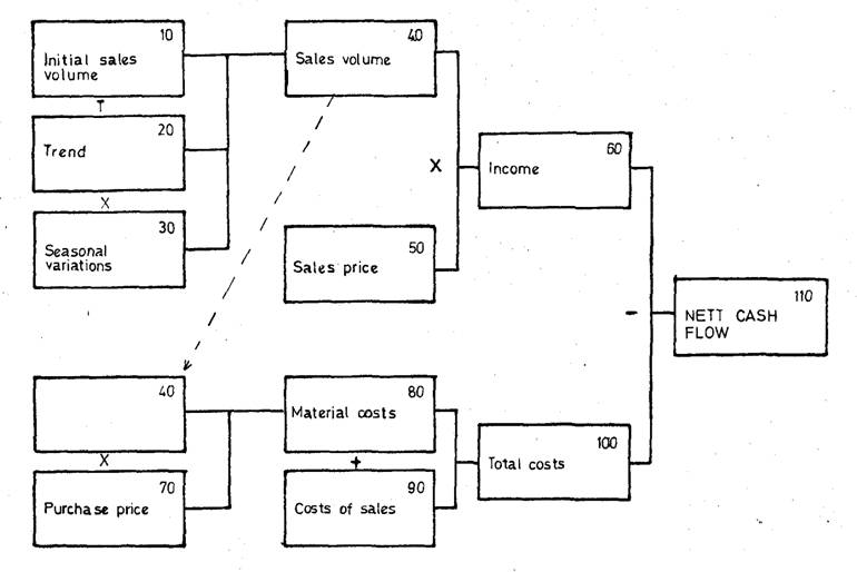
Figure 2 – The code

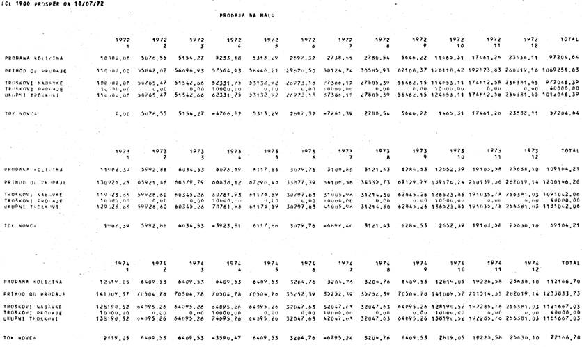
Figure 3 – A part of the output

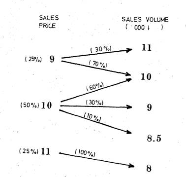
Figure 4 – Dependencies

Note - arrows indicate dependencies and numbers in brackets probabilities